![]()
Contents |
 |
![]()
Learning vector quantization is a precursor of the well-known self-organizing maps (also called Kohonen feature maps) and like them it can be seen as a special kind of artificial neural network. Both types of networks represent a set of reference vectors, the positions of which are optimized w.r.t. a given dataset. Note, however, that this document cannot provide an exhaustive explanation of learning vector quantization (see a textbook on neural networks for that). Rather, it only briefly recalls the basic ideas underlying this kind of neural networks.
A neural network for learning vector quantization consists of two layers: an input layer and an output layer. It represents a set of reference vectors, the coordinates of which are the weights of the connections leading from the input neurons to an output neuron. Hence, one may also say that each output neuron corresponds to one reference vector.
The learning method of learning vector quantization is often called competition learning, because it works as follows: For each training pattern the reference vector that is closest to it is determined. The corresponding output neuron is also called the winner neuron. The weights of the connections to this neuron - and this neuron only: the winner takes all - are then adapted. The direction of the adaption depends on whether the class of the training pattern and the class assigned to the reference vector coincide or not. If they coincide, the reference vector is moved closer to the training pattern, otherwise it is moved farther away. This movement of the reference vector is controlled by a parameter called the learning rate. It states as a fraction of the distance to the training pattern how far the reference vector is moved. Usually the learning rate is decreased in the course of time, so that initial changes are larger than changes made in later epochs of the training process. Learning may be terminated when the positions of the reference vectors do hardly change anymore.
| back to the top |  |
![]()
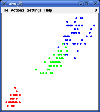
Visualizing learning vector quantization is obviously very simple, as long as we confine ourselves to two input attributes plus an optional class attribute. In this case we can draw a scatterplot of the training patterns. As an example the picture below shows the well-known iris data for the attributes petal_length (horizontal) and petal_width (vertical). The color of the data points indicates the class: red - iris setosa, green - iris versicolor, and blue - iris virginica. (A data file containing the iris data in a format that can be read with the default data format specification can be found in the directory ex of the source package.)
 |
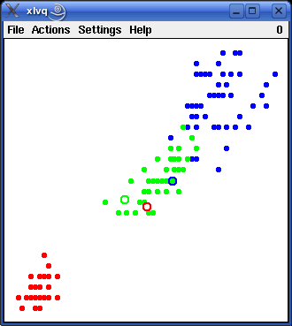
In the same way we can visualize the reference vectors, which are also points in the data space. By selecting the menu entry Actions > Initialize a set of three reference vectors is generated - one per class (the number of reference vectors per class can be changed in the parameters dialog box, see below). These vectors are shown as small circles in the left picture below.
 |
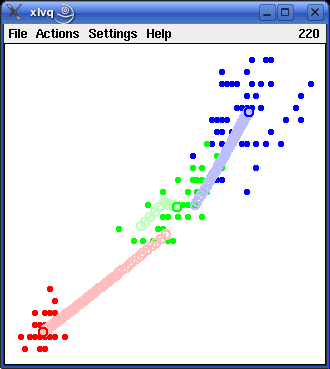 |
As a next step training can be started by selecting the menu entry Actions > Start Training. When this is done, each reference vector moves towards the group of training patterns that have the same class as that assigned to it. To make this movement easier to follow, the previous positions of the reference vectors are not erased, but drawn in a lighter shade of the corresponding color. The result is shown in the right picture above.
The above example used the class information present in the attribute iris_type. However, learning vector quantization may also be applied when no class information is available, by simply treating all training patterns as belonging to the same class. Of course, in this case the number of reference vectors per class should be increased. The two pictures below show the initialization and the training of three reference vectors (shown as red circles).
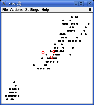 |
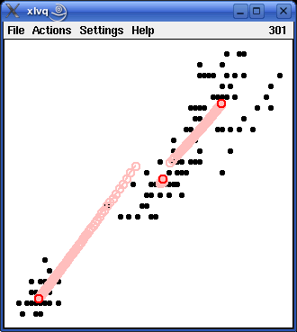 |
If the two learning results shown above - one using the class information and one neglecting it - are studied in detail, it turns out that they are very similar, but that with the class information taken into account the vectors for the iris versicolor patterns and the iris virginica patterns are somewhat farther apart from each other than when the class information is neglected. The reason is that reference vectors are repelled if they are closest to a training pattern belonging to a different class. This "repel rule" is applied in case the class information is taken into account, because the training patterns for iris versicolor and iris virginica are not cleanly separated. If the class information is neglected, however, the "repel rule" is - obviously - never applied.
| back to the top | |
![]()
The programs xlvq and wlvq always work on data loaded from a file. In order to provide some flexibility w.r.t. the file formats that can be read, some properties of the data format can be specified in the dialog box that is opened, when the menu entry File > Data Format... is selected. This dialog box is shown below.
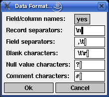
The idea underlying this data format specification is that a data file basically consists of a set of records, each describing a tuple and consisting of a set of data fields. This structure is brought about by three types of special characters: blanks, field separators and record separators. The meaning of these types of characters is described in the list below. All text input fields accept the standard ASCII escape sequences like `\t' for the tabulator or `\177' or '\x7f' for the delete character.
| First record contains: | The contents of the first record of the data file: Either attributes (meaning the names of attributes), data (meaning attribute values), or comments. If "comments" is chosen, the first record is simply ignored and the second record is assumed to hold attribute names. | |
| Blank characters: | Characters that are used to fill a field, possibly to align it, but that should not be read as part of the attribute name or attribute value. These characters are removed when the data file is read. The default comprises the carriage return character `\r' in order to avoid problems with DOS/Windows text files under Unix. | |
| Field separators: | Characters that separate two fields (attribute values) within a record (data tuple). The default is the space and the tabulator, which is usually appropriate for ASCII text tables. | |
| Record separators: | Characters that separate two records (data tuples) from each other. The default is a newline character, which is usually appropriate for ASCII text tables. | |
| Unknown value characters: | Characters that are used to identify unknown attribute values. The contents of a data field is assumed to represent an unknown value if it consists entirely of blank characters and the characters specified in this field. |
The learning process of the learning vector quantization is influenced by several parameters. If the menu entry Settings > Parameters... is selected (or, in the Unix version, if `p' for `parameters' is pressed), a dialog box is opened in which these parameters can be changed (this dialog box is shown below).
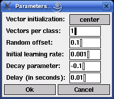
| Vector initialization: | This field controls how the reference vectors are initialized. There are four choices: They may be set to the centers of the ranges of values of the two input attributes, to the global mean of the data w.r.t. these two attributes, to the means per class, or to a randomly chosen data point (of the corresponding class). | |
| Vectors per class: | The number of reference vectors that are used per class. It is only possible to state this number globally, i.e., the same number of vectors is used for all classes. The default is 1. | |
| Random offset: | The initial coordinates of the reference vectors are modified by adding a random offset from the interval [-x,+x]. In this field the value of x can be entered. The default is 0.1. | |
| Initial learning rate: | In learning vector quantization the learning rate states the fraction of the distance between a data point and the closest reference vector. It determines how far the reference vector is moved towards or away from the data point. The default value is eta0 = 0.001, i.e., the reference vector is moved 0.001 times the distance to the data point. | |
| Decay exponent: | The learning rate is decreased in the course of time according to the formula eta(t) = eta0tk (if k is negative) or according to the formula eta(t) = eta0kt (if k is positive). In this field the value of k can be entered. The default is -0.01. | |
| Delay (in seconds): | The time between two consecutive training epochs (one epoch: one traversal of all training patterns). By enlarging this value the training process can be slowed down or even executed in single epochs. The default is 0.01 seconds. |
All entered values are checked for plausibility. If a value is entered that lies outside the acceptable range for the parameter (for example, a negative learning rate), it is automatically corrected to the closest acceptable value.
The programs xlvq and wlvq take at most two attributes as input for the learning vector quantization, namely the two attributes assigned to the two coordinate axes of the scatterplot displayed in the program window. In addition to these two attributes, information about a class value may enter the computations (see above). However, data tables loaded into the program may contain more than 2 or 3 columns. Which of the attributes present in a loaded data table shall be used as inputs and which as the class attribute can be specified by selecting the menu entry Settings > Attributes... (or, in the Unix version, by simply pressing `t'). This opens the dialog box shown below (here with the attributes for the iris data).
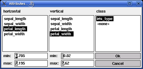
Note that the two list boxes on the left show only attributes that have been recognized as numeric, whereas the list box on the right shows only attributes that have been recognized as symbolic. Hence only numeric attributes can be selected as inputs and only a symbolic attribute can be selected as the class attribute. The class attribute may also be deselected if it is not to be used for training. To do so, one may select the special entry <none>.
The two input fields min and max below the list boxes for the horizontal and the vertical attribute show an (enlarged) range of values for the currently selected attributes. These values are computed from the actual minimal and maximal value of the attribute occurring in the loaded data by enlarging the difference between these values by 10%. The values in these fields may be changed in order to control the area that is displayed in the window. However, changed values are not stored with the attributes, but apply only to the current diagram.
Selecting the menu entry Settings > Colors (or, in the Unix version, simply pressing `c' for `colors') opens the dialog box shown below. It allows a minimal control of the colors used to display the data and the reference vectors.
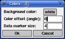
The first field states the background color, which may be either black or white. The second field controls the selection of the class colors w.r.t. a standard color circle. 0 degrees correspond to the color red, 120 degrees to the color green and 240 degrees to the color blue. Class color angles are chosen according to the formula ci = o +360i/n, where i is the class index, n is the number of classes and ci the color angle for the class with index i. o is the offset that may be entered in the second input field.
Sets of reference vectors can also be saved to a file and reloaded later. To do so one has to select the menu entries File > Save Vectors... or File > Load Vectors..., respectively. (Alternatively, in the Unix version, one may press `s' for `save' and `l' for `load'.) The file selector box that is opened, if one of these menu entries are selected, is shown below. (In the Windows version the standard Windows file selector box is used.)
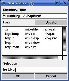
The edit field below 'Directory/Filter' shows the current path, the list box below 'Files' the files in the current directory matching the current file name pattern. (A file name pattern, which may contain the usual wildcards '*' and '?', may be added to the path. When the file name pattern has been changed, pressing the 'Update' button updates the file list.) The line below 'Selection' shows the currently selected file. It may be chosen from the file list or typed in.
| back to the top | |
![]()
(MIT license, or more precisely Expat License; to be found in the file mit-license.txt in the directory lvqd/doc in the source package, see also opensource.org and wikipedia.org)
© 2000-2016 Christian Borgelt
Permission is hereby granted, free of charge, to any person obtaining a copy of this software and associated documentation files (the "Software"), to deal in the Software without restriction, including without limitation the rights to use, copy, modify, merge, publish, distribute, sublicense, and/or sell copies of the Software, and to permit persons to whom the Software is furnished to do so, subject to the following conditions:
The above copyright notice and this permission notice shall be included in all copies or substantial portions of the Software.
THE SOFTWARE IS PROVIDED "AS IS", WITHOUT WARRANTY OF ANY KIND, EXPRESS OR IMPLIED, INCLUDING BUT NOT LIMITED TO THE WARRANTIES OF MERCHANTABILITY, FITNESS FOR A PARTICULAR PURPOSE AND NONINFRINGEMENT. IN NO EVENT SHALL THE AUTHORS OR COPYRIGHT HOLDERS BE LIABLE FOR ANY CLAIM, DAMAGES OR OTHER LIABILITY, WHETHER IN AN ACTION OF CONTRACT, TORT OR OTHERWISE, ARISING FROM, OUT OF OR IN CONNECTION WITH THE SOFTWARE OR THE USE OR OTHER DEALINGS IN THE SOFTWARE.
| back to the top | |
![]()
Download page with most recent version.
| back to the top | |
![]()
| E-mail: |
christian@borgelt.net | |
| Website: |
www.borgelt.net |
| back to the top | |
![]()