![]()
Contents |
 |
![]()
Artificial neural networks are often seen as black boxes which compute in a mysterious way one or more output values for a vector of input values. How they are trained by backpropagation to represent a certain function is usually considered to be even more mysterious and only justifiable by complex mathematical means. However, if the learning problem and the network structure are simple enough, it is possible to visualize the computations of the network and how these computations change due to training. The programs xmlp (Unix/X11) and wmlp (Windows) visualize the training process of very simple so-called multi-layer perceptrons for two logical and two simple real-valued functions.
For a logical function (also called a Boolean function, in honor of George Boole, 1815-1864) like, for instance, the logical 'and', the basic idea of the visualization is that each neuron (except the input neurons) can be seen as representing a separating line, plane, or hyperplane in the corresponding input space. (Of course, this is strictly correct only for crisp thresholds. However, only little harm is done if this view is transferred to sigmoid activation functions, at least if we are concerned only with logical functions.) This line, plane, or hyperplane separates those points of the input space for which an output value of 1 is desired from those points for which an output value of 0 is desired. Obviously, this interpretation allows us to visualize the computations of a neuron with two or three inputs by simply drawing the represented separating line or plane in an appropriate coordinate system.
For a real-valued function the basic idea of the visualization is that the "slopes" of the function are approximated by the sigmoid activation functions of the neurons in the hidden layer. Since an output neuron computes a weighted sum of its inputs, it can be seen as "joining the slopes" represented by the neurons in the hidden layer. Obviously, this view also allows for a simple visualization of the computations of the neurons, provided there are only one or two input variables.
| back to the top |  |
![]()
A good choice for Boolean functions to learn are the exclusive or and the biimplication, because these two functions are the simplest problems in which the input vectors, for which different output values are desired, are not linearly separable (i.e., there is no single line separating them). Therefore a single neuron is not enough to solve these problems. A multi-layer perceptron is needed. However, a very simple multi-layer perceptron with only five neurons (two input neurons, two hidden neurons, and one output neuron) suffices. This network is simple enough so that its computations can be visualized, because no neuron has more than two inputs.
| back to the top | |
![]()
When the visualization program is invoked, a window is opened that looks like the one shown in the picture below. (All screenshots were obtained from xmlp, the Unix version of the program, with the Unity Desktop of Ubuntu GNU/Linux.)
The window is split into an upper and a lower part. The upper part shows the neural network with its five neurons in a standard representation. The two grey circles on the left are the input neurons, the magenta and the turquoise circle in the middle are the neurons of the hidden layer, and the orange circle on the right is the output neuron. The arrows between these circles indicate the connections. The numbers printed over these arrows are the connections weights, the numbers printed below or atop of the circles are the threshold values of the corresponding neurons. For example, in the picture below the upper (magenta) hidden neuron is connected with a weight of -0.4433 to the lower input neuron and with a weight of 0.208 to the upper input neuron. Its threshold value is -0.348.
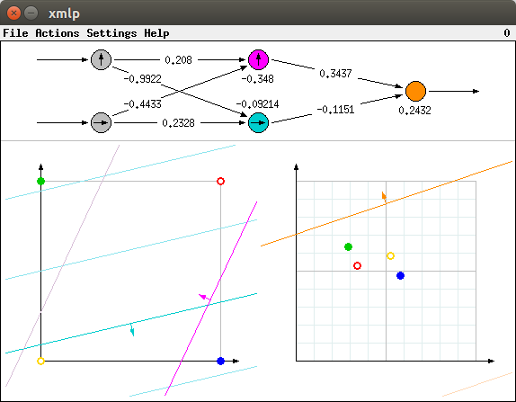
The lower part of the window shows the input spaces of the neurons of the hidden layer (left diagram) and of the output neuron (right diagram). The arrows in the circles representing the neurons in the upper part of the window indicate how the output values of these neurons are associated with the coordinate axes of these diagrams. The lower input neuron is associated with the horizontal axis of the left diagram, the upper input neuron with the vertical axis. Likewise, the lower (turquoise) hidden neuron is associated with the horizontal axis of the right diagram and the upper (magenta) hidden neuron is associated with the vertical axis.
In addition, the lower (turquoise) hidden neuron is associated with the turquoise lines, the upper (magenta) hidden neuron with the magenta lines in the left diagram. Likewise, the (orange) output neuron is associated with the orange lines in the right diagram. Those of these lines that have full color saturation and a small arrow attached to them are the separating lines represented by the connection weights and the threshold values of these neurons. (More precisely, these lines indicate the points in the input spaces at which the logistic function of the corresponding neuron has a value of 0.5, see below). These lines are computed as follows: The weights of the input connection of a neuron are the coordinates of the normal vector of its separating line. In the diagrams these normal vectors are indicated by small arrows in the middle of the lines. The threshold value of a neuron determines the distance of its separating line from the origin (w.r.t. the normal vector of the line). If the threshold is negative, then the origin is on the same side of the line as the normal vector, otherwise it is on the other side. The distance of the origin (i.e., the length of a perpendicular line from the origin to the separating line) is the threshold value divided by the length of the normal vector.
In this way the weighted sum of the coordinates of a point in the input space of a neuron minus the threshold value is zero if and only if this point lies on the separating line (or 0.5 line, see below). It is positive if the point lies on that side of the line the normal vector points to, otherwise it is negative. Therefore, with a crisp threshold function the neuron would yield an output value of 1 for all points on the separating line and all points on that side of its separating line the normal vector of this line points to. For all other points the output value is 0.
Of course, if we want to train a neural network with the standard backpropagation method, we cannot use crisp thresholds, but we have to use a sigmoid activation function, since the activation function must be differentiable. (See the next section on real-valued functions for pictures of sigmoid functions.) With such a function the output value of a neuron is 0.5 for points on its separating line (which is better called a characteristic line in this case). For points on that side of the line the normal vector points to the output is greater than 0.5, on the other side it is less than 0.5. Obviously, the further away a point is from the characteristic line, the more its corresponding output value differs from 0.5. Hence the function computed by a neuron is a curved ascending surface with its gradient in the direction of the normal vector of the characteristic line.
To make it easier to imagine this curved behavior, a few additional contour lines of the logistic function are shown. In principle, the visualization program shows contour lines for the values 0.1 to 0.9 in steps of 0.1, of which the 0.5 line is shown with full color saturation (and with the normal vector indicating the direction of ascent attached to it), while all other contour lines are shown with reduced color saturation. However, in the initial situation that is depicted in the above picture, only some additional contour lines are visible, namely those for 0.3, 0.4, and 0.6 for the turquoise neuron, that for 0.6 for the magenta neuron and that for 0.4 for the orange neuron (lower right corner of right diagram).
With the above considerations the computations of the two neurons in the hidden layer of the neural network can be seen as a coordinate transformation. For each point of the input space they compute two output values, both in the range [0,1]. These output values can be interpreted as the coordinates of a point in the input space of the output neuron. The output neuron then computes its output value from the transformed coordinates.
As an illustration consider the four points of the input space that are used for the exclusive or and the biimplication problem, namely the corners of the unit square. These four points are shown as small colored circles in the left diagram of the lower part of the window: yellow - (0,0), blue - (1,0), green - (0,1), and red - (1,1). The picture above shows the 'exclusive or' problem, as can be seen from the fact that the blue and the green circle are solid, indicating that for these points an output value of 1 is desired. In contrast to this the yellow and the red circle are shown as rings, indicating that for these points an output value of 0 is desired.
The transformed points are shown with the same colors in the right diagram. Their positions can be made plausible as follows (drawing on those additional contour lines that are visible in the left diagram): The yellow and the blue point lie on that side of the (fully saturated) turquoise line the normal vector of this line points to. Hence the output value of the lower (turquoise) hidden neuron should be greater than 0.5. In contrast to this, the output value of the turquoise neuron should be less than 0.5 for the green and the red point. Since the lower (turquoise) neuron corresponds to the horizontal axis of the right diagram, the yellow and the blue point should be mapped to the right of the vertical grey line in the middle of this diagram (the 0.5 line - it corresponds directly to the turquoise line in the left diagram), whereas the red and the green point should be mapped to the left of this line. Actually this is the case.
Note that the additional (less saturated) additional contour lines allow for a more precise determination of the destination location. The yellow point is closer to the turqouise 0.5 line, while the blue point is closer to the additional (less saturated) 0.6 turquoise contour line, explaining their position relative to the vertical grid lines in the right diagram. Likewise, the green point is just before the additional 0.3 turquoise contour line, the red point between the 0.3 and 0.4 contour lines. Analogously the vertical positions can be made plausible by considering the positions of these points relative to the (fully saturated) 0.5 magenta and the additional (less saturated) 0.6 contour line.
| back to the top | |
![]()
Obviously, for the simple logical functions we are concerned with here, the task of training the network is to find a transformation of the input coordinates that makes it is possible to find a separating line for the transformed points. Such a transformation is indeed found for the initial configuration shown above if the network is trained with backpropagation.
Network training can be started by selecting the menu entry Actions > Start Training (or, in the Unix version, by simply pressing 'x' for 'execute'). Then the connection weights of the network are changed and the separating lines (0.5, fully saturated colors) as well as the additional lines (less saturated colors) are shifted correspondingly. In addition the transformed points in the right diagram move to new positions, depending on the positions of the colored lines in the left diagram. The epochs, i.e., the number of times the training patterns have been presented to the network, are shown in the upper right corner of the window (in the menu bar, in the Windows version this number is shown in the title bar of the window). Eventually the situation is reached that is shown in the picture below. Then training may be stopped by selecting Actions > Stop Training (or, in the Unix version, by simply pressing 'x' again).
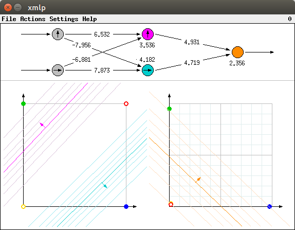
Obviously the training process was successful. The colored lines in the left diagram each separate one of the points, for which an output value of 1 is desired, from all other points. Hence the blue point is the only one for which the horizontal coordinate in the right diagram is (close to) 1, since it is the only one which lies on that side of the (fully saturated) turquoise line the normal vector of this line points to. And since it lies beyond the 0.9 turquoise contour line, but far before the 0.1 magenta contour line, it is clear that it must be close to the bottom right corner of the right diagram. For all other points the horizontal coordinate is (close to) 0, as they lie (far) before the 0.1 turquoise contour line.
Likewise, the green point is the only one for which the vertical coordinate is (close to) 1, since it is the only one that lies on that side of the (fully saturated) magenta line the normal vector of this line points to. And since it lies beyond the 0.9 magenta contour line, but far before the 0.1 turquoise contour line, it is clear that it must be close to the upper left corner of the right diagram. For all other points the vertical coordinate is (close to) 0, as they lie (far) below the 0.1 magenta contour line.
As a consequence, both points for which an output value of 0 is desired, namely the yellow and the red point, are mapped (close) to the origin of the right diagram (the yellow point is almost hidden under the red point), whereas both points for which an output value of 1 is desired are mapped (close) to (1,0) and (0,1). This makes it possible to separate the points by the (fully saturated) orange line as shown in the picture above. Note that the blue and the green point lie on that side of this orange line the normal vector of this line points to. And since they are just beyond the 0.9 orange contour line, the output values for these points are (close to) 1, while the output values for the yellow and the red point are (close to) 0, as they lie just before the 0.1 orange contour line.
Note that the absolute values of the connection weights are much larger as in the initial configuration. These higher values explain why all additional contour lines are much closer together (and are thus all visible) and why the distances of the transformed points from the 0.5 lines are so much larger than in the initial configuration, although the distances of the corresponding points from the colored lines in the left diagram is comparable to the initial configuration. Intuitively, the sigmoid activation functions get steeper as (the absolute values of) the weights get larger (see also below, where this is shown more clearly in connection with the approximation of real-valued functions).
Although the training process is often successful, resulting in configurations similar to the one shown above, there are situations in which it fails. Depending on the initialization, the training process may lead to a situation like the one shown in the picture below.
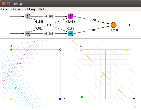
Obviously the training was not successful. Although for the yellow and the green point the correct values (close to 0 and close to 1, respectively) are computed, for both the red and the blue point (the latter is hidden under the red one), an output value of (about) 0.5 is computed, since both points lie on (or rather very close to) the separating line (the fully saturated orange line, representing the points where the logistic function is 0.5). This shows that the training can get stuck in a local minimum of the error function.
The network weights may be reinitialized any time, even during training, by selecting one of the menu entries Actions > Exclusive or or Actions > Biimplication. (Alternatively, in the Unix version, one may press `e' for `exclusive or' and `b' for `biimplication'.)
| back to the top | |
![]()
Since a real-valued function is learned by an artificial neural network by approximating the "slopes" of this function by the sigmoid activation functions of the hidden neurons (see above), functions with few clear slopes are a good choice. In the programs xmlp and wmlp a trapezoid function (with slopes of different gradient) and a ascending function (with a changing gradient) are used.
| back to the top | |
![]()
If one of the menu entries Actions > Function 1 (trapezoid function) or Actions > Function 2 (ascending function) is selected, a different neural network and a different diagram are drawn. If Function 1 is selected, the window should look like the one shown in the picture below. As for the Boolean functions the window is split into two parts, with the neural network in the upper part and the diagram in the lower. However, the neural network has only one input and there is only one diagram.
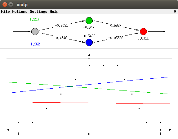
The horizonal axis of the diagram corresponds to the input variable. It ranges from -1 (left tick) to 0 (vertical axis) to +1 (right tick). The vertical axis corresponds to the output variable. It ranges from 0 (horizontal axis) to 0.5 (lower grey line) to 1 (upper grey line). The black dots in the diagram are the training patterns. They define the function the network is to learn. The colored lines indicate the output of the different neurons for different input values. As for the Boolean functions each colored line corresponds to the neuron with the same color. That is, the blue and the green line correspond to the neurons of the hidden layer, the red line corresponds to the output neuron. Since the network is freshly initialized with rather small random weights, these lines are almost straight. That the blue and the green line actually represent the sigmoid activation functions of the hidden neurons and that the red line is an aggregate of the two will become obvious when the network is trained.
| back to the top | |
![]()
When the network is trained, the sigmoid functions (the blue and the green line) become steeper and are adapted to the "slopes" of the trapezoid function. The network output (red line) is computed as an aggregate of the two. The learning result that is obtained with the initialization shown above is shown in the picture below.
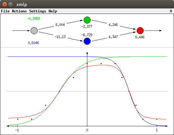
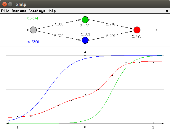
The sigmoid functions of this diagram (blue and green line) are connected to the network weights as follows: The threshold value of the corresponding neuron divided by its input connection weight is the value on the horizontal axis for which the sigmoid function has the value 0.5. For example, for the green line the threshold -2.377 divided by the input connection weight 6.004 is about -0.3959 (shown in green above the input neuron). This is the value for which green line crosses the lower grey line (the 0.5 line). Likewise, for the blue line the threshold -6.729 divided by the input connection weight of -11.13 is about 0.6046 (shown in blue below the input neuron). This is the value for which blue line crosses the lower grey line (the 0.5 line).
The gradient of the sigmoid functions is controlled by the (absolute value of the) input weight: The higher the (absolute value of the) weight, the steeper the function. Compare, for instance, the gradient of the green line (input weight 6.004) to the gradient of the blue line (input weight -11.13): The latter is steeper than the former.
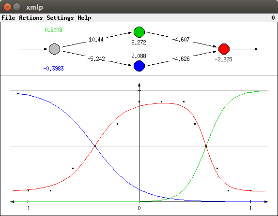
Note that the sigmoid activation functions of the hidden neurons need not have the same "direction" as the "slopes" of the output function as in the picture above. If the weight of the connection to the output neuron is negative, the gradient is inverted. In such a case we may get a learning result as the one shown in the picture below. Of course, we may also end up with a network in which one of the hidden neurons conforms to the gradient of the output function whereas the other is inverted.
As for the Boolean functions, the training can get stuck in a local minimum of the error function. One such situation is shown in the picture below. Obviously, the training was not successful. Although it can be seen that an attempt was made to approximate the left slope, the right slope is completely neglected. Consequently the network output (red line) does not fit the data well.
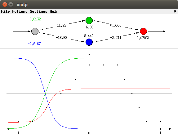
A learning result for the second real-valued function (selectable with Actions > Function 2) is shown below. Obviously, the neural network achieved a very good fit to the data.
As for the Boolean functions the network weights may be reinitialized any time, even during training, by selecting one of the menu entries Actions > Function 1 or Actions > Function 2. (Alternatively, in the Unix version, one may press `1' for `function 1' and `2' for `function 2'.)
| back to the top | |
![]()
The learning process of the neural network is influenced by several parameters. If the menu entry Settings > Parameters... is selected (or, in the Unix version, if `p' for `parameters' is pressed), a dialog box is opened in which these parameters can be changed (this dialog box is shown below).
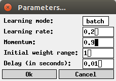
| Learning mode: | Either 'online' (update weights after each pattern) or 'batch' (update weights after one traversal of all patterns with the aggregated changes). The default is batch, since it leads to a smoother training behavior. | |
| Learning rate: | The severity of the weight changes relative to the computed network error. A higher learning rate can speed up training. However, if the learning rate is too large, training may fail completely. Often a value of 0.2, which is the default, is recommended. However, moderately larger values seem to work well, too. | |
| Momentum: | The proportion of the weight change of the previous training step that is transferred to the next step. This models some kind of inertia in the gradient descent, which can speed up training. The value of this parameter should be less than 1. A value of 0.9 is a good choice, but the default is 0 (standard backpropagation without momentum). | |
| Initial weight range: | The initial connection weights are chosen from an interval [-x,+x]. In this field the value of x may be entered. The default is 1. | |
| Delay: | Time between two consecutive training steps. By enlarging this value the training process can be slowed down or even executed in single steps. The default is 0.01 seconds. |
All entered values are checked for plausibility. If a value is entered that lies outside the acceptable range for the parameter (for example, a negative learning rate), it is automatically corrected to the closest acceptable value.
If the menu entry Settings > Weights... is selected (or, in the Unix version, if `w' for `weights' is pressed), a dialog box is opened in which the connection weights and the threshold values of the output neuron and the two neurons in the hidden layer may be entered (this dialog box is shown below).
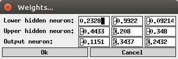
Each line of this dialog box corresponds to one neuron. The first two fields in each line are the weights of the input connections of the corresponding neuron: For a Boolean function the first field corresponds to the horizontal direction of the input space, the second to the vertical direction. For a real-valued function the first input field for a hidden neuron corresponds to the input connection weight whereas the second input field is neglected (it is set to 0 in this case). The last field contains the threshold value of the neuron.
The weights of the neural network can also be saved to a file and reloaded later. To do so one has to select the menu entries File > Save Weights or File > Load Weights, respectively. (Alternatively, in the Unix version, one may press `s' for `save' and `l' for `load'.) The file selector box that is opened, if one of these menu entries are selected, is shown below. (The Windows version uses the standard Windows file selector box.)
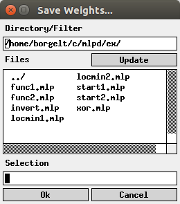
The edit field below 'Directory/Filter' shows the current path, the list box below 'Files' the files in the current directory matching the current file name pattern. (A file name pattern, which may contain the usual wildcards '*' and '?', may be added to the path. When the file name pattern has been changed, pressing the 'Update' button updates the file list.) The line below 'Selection' shows the currently selected file. It may be chosen from the file list or typed in.
| back to the top | |
![]()
(MIT license, or more precisely Expat License; to be found in the file mit-license.txt in the directory mlpd/doc in the source package, see also opensource.org and wikipedia.org)
© 1999-2017 Christian Borgelt
Permission is hereby granted, free of charge, to any person obtaining a copy of this software and associated documentation files (the "Software"), to deal in the Software without restriction, including without limitation the rights to use, copy, modify, merge, publish, distribute, sublicense, and/or sell copies of the Software, and to permit persons to whom the Software is furnished to do so, subject to the following conditions:
The above copyright notice and this permission notice shall be included in all copies or substantial portions of the Software.
THE SOFTWARE IS PROVIDED "AS IS", WITHOUT WARRANTY OF ANY KIND, EXPRESS OR IMPLIED, INCLUDING BUT NOT LIMITED TO THE WARRANTIES OF MERCHANTABILITY, FITNESS FOR A PARTICULAR PURPOSE AND NONINFRINGEMENT. IN NO EVENT SHALL THE AUTHORS OR COPYRIGHT HOLDERS BE LIABLE FOR ANY CLAIM, DAMAGES OR OTHER LIABILITY, WHETHER IN AN ACTION OF CONTRACT, TORT OR OTHERWISE, ARISING FROM, OUT OF OR IN CONNECTION WITH THE SOFTWARE OR THE USE OR OTHER DEALINGS IN THE SOFTWARE.
| back to the top | |
![]()
Download page with most recent version.
| back to the top | |
![]()
| E-mail: |
christian@borgelt.net | |
| Website: |
www.borgelt.net |
| back to the top | |
![]()